Principal Component Analysis of the S&P 500: Eigenportfolios vs. Passive Investing

Read the full paper (PDF) · Code and data on GitHub

Summary

I ran Principal Component Analysis on five years of daily adjusted closing prices for S&P 500 constituents, July 2021 to March 2026, to find the hidden factors behind equity returns. I then turned the components into long-only portfolios and backtested them against SPY. Three of four strategies delivered better risk-adjusted returns than the index, though a bootstrap shows none of the gaps is statistically significant. PC4, which captures AI infrastructure against housing, reached a Sharpe ratio of 0.76 against 0.38 for SPY. A combined four-factor portfolio had the lowest drawdown of any strategy tested, at -14.7%.

Why PCA

A market-cap weighted index gives you every factor risk at once, with no way to lean toward the attractive ones or away from the rest. PCA breaks a large return matrix into orthogonal factors, each an independent source of movement across stocks. After interpreting those factors, you can build portfolios that concentrate in specific ones. These are eigenportfolios.

Data and method

• Prices: daily adjusted closes from Yahoo Finance (yfinance), checked against FactSet’s Universal Screener, pulled for March 9, 2021 to March 9, 2026.
• Cleaning: tickers missing more than 10% of observations were dropped, leaving 495 stocks. Prices were converted to daily log returns, r = ln(P_t / P_t−1), keeping only days on which every stock traded. Because the latest listing (HOOD) began trading in late July 2021, the working sample is 1,155 trading days, July 30, 2021 to March 6, 2026.
• Standardization: every stock scaled to mean 0 and standard deviation 1, so high-volatility names like semiconductors don’t dominate the components just because their numbers are larger.
• PCA: 50 components extracted from the standardized 1,155 × 495 matrix.
• Eigenportfolios: each component’s loadings used as raw weights, negatives set to zero (long-only), the rest normalized to sum to one. Weights fixed at the start, no rebalancing, 4% risk-free rate.

What the components mean

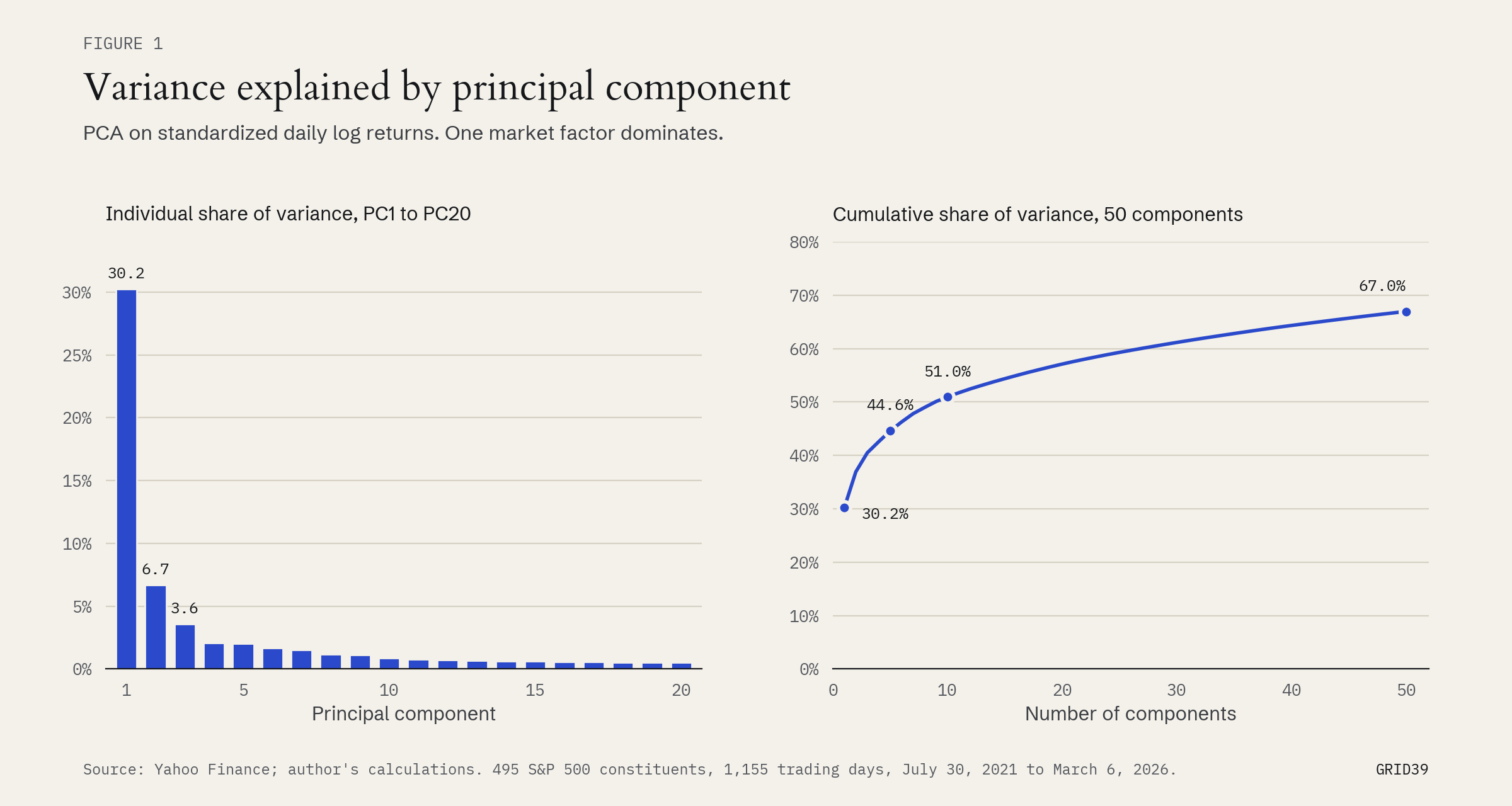
PC1 alone explains 30.2% of return variance, and the drop after it is steep. Even 50 components reach only about 67%; the rest is mostly stock-specific noise that diversification handles.

Component	Variance	Positive side	Negative side
PC1	30.2%	Market factor: almost every stock, led by BLK, AMP, ITW	Lowest loadings: KR, DG, MCK
PC2	6.7%	Regulated utilities (ED, DUK)	Semiconductors (NVDA, LRCX, AMAT)
PC3	3.6%	Oil and gas (COP, XOM, HAL, SLB)	High-multiple software (INTU, NOW, ADBE)
PC4	2.1%	AI infrastructure and power (VST, WMB, NVDA, CRWD, ANET)	Homebuilders and materials (LEN, DHI, SWK, MAS)
PC5	2.0%	P&C insurers (ACGL, AJG, CB, PGR)	Rate-sensitive utilities and REITs (DLR, NEE, CMS)

PC2 likely reflects interest-rate sensitivity. PC3 is the inflation trade: rising prices boosted energy cash flows while compressing software multiples. PC4 is the most interesting given the sample period, since it captures the defining macro trends of 2022 to 2025.

Backtest results

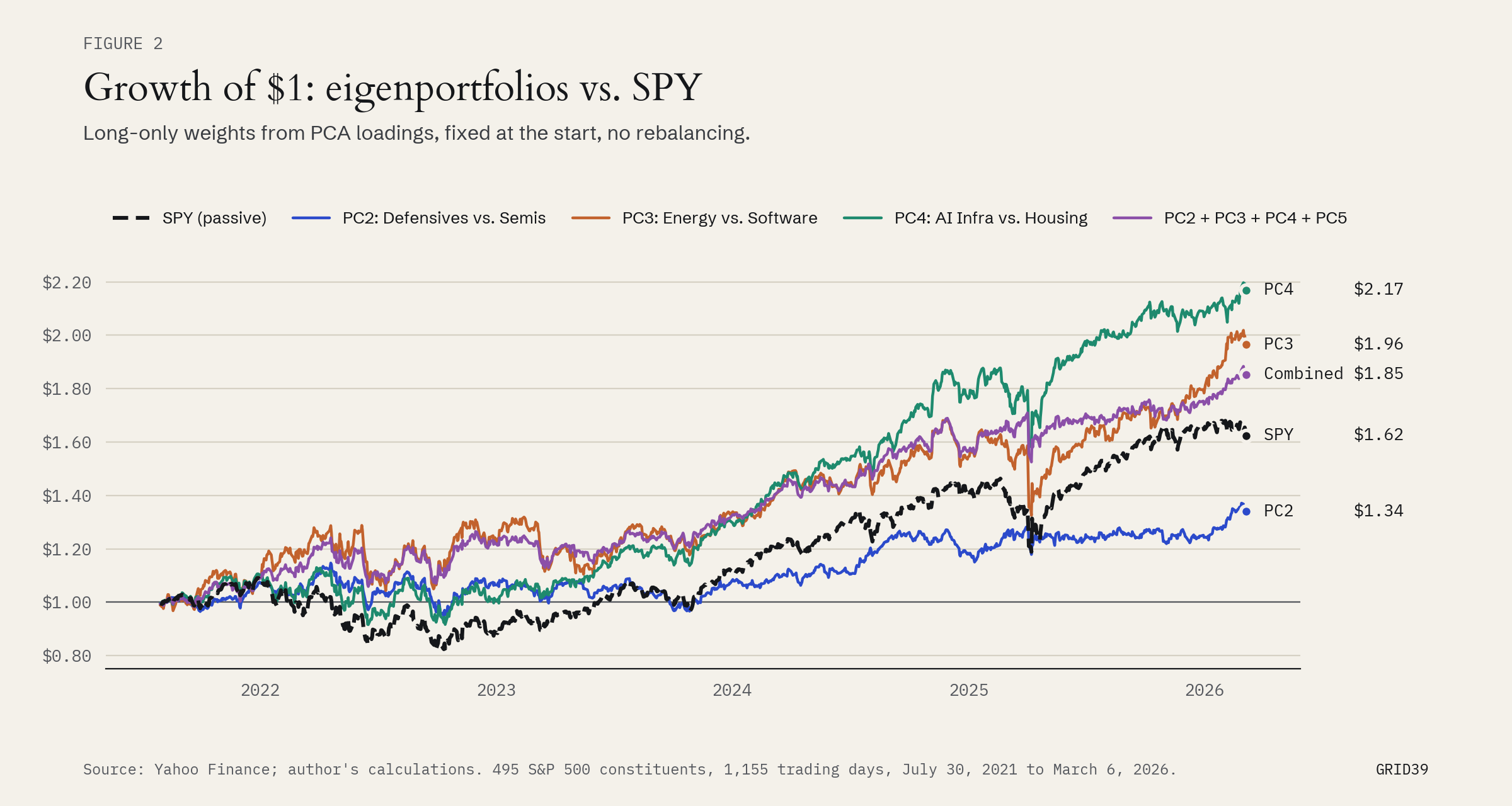
Portfolio	Ann. return	Volatility	Sharpe	Max drawdown	Total return
SPY (passive)	11.2%	17.3%	0.38	-24.5%	62.4%
PC2: Defensives vs. Semis	6.6%	13.2%	0.18	-17.4%	33.9%
PC3: Energy vs. Software	15.9%	19.8%	0.54	-21.3%	96.5%
PC4: AI Infra vs. Housing	18.4%	17.0%	0.76	-18.9%	116.9%
PC2 + PC3 + PC4 + PC5	14.4%	14.1%	0.67	-14.7%	85.3%

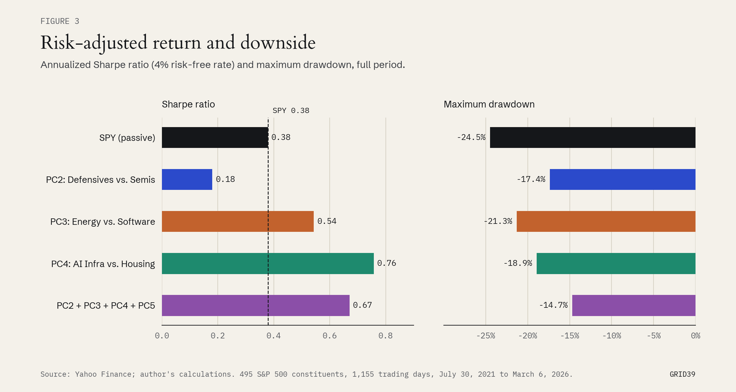
PC4 was the strongest single factor: more return than SPY with a smaller drawdown. Leaning into AI infrastructure and power-grid names while avoiding homebuilders produced the highest total return of the period.

PC3 also beat SPY on a risk-adjusted basis, helped by the 2021 to 2022 commodity cycle and the rerating of energy cash flows as inflation rose.

PC2 underperformed badly. Utilities were hit hard by rising rates through 2022 and 2023. It shows the central risk: picking the wrong factor at the wrong point in the cycle can be worse than owning the index.

The combined portfolio is arguably the most useful result. Blending four orthogonal components gave a 0.67 Sharpe and a -14.7% maximum drawdown, the lowest of any strategy, SPY included. That is what factor diversification looks like in practice.

Limitations

• In-sample. Loadings were computed on the same 2021 to 2026 window used to measure performance. A rigorous test would roll forward: fit PCA on 36 months, test on the next 12, repeat.
• No transaction costs. Eigenportfolios need rebalancing as loadings shift. At 30 to 50% annual turnover, net returns would be meaningfully lower.
• Survivorship bias. The universe is today’s S&P 500, so companies dropped or delisted during the period are missing. That biases every strategy upward.
• Sampling uncertainty. A Sharpe ratio from under five years of data is a noisy estimate. A block bootstrap (below) shows the gaps to SPY are not statistically significant.

How certain are the results?

To test whether the Sharpe ratios are distinguishable from SPY’s, I resampled each portfolio’s daily returns with a fixed-block bootstrap: 20-day blocks, to keep volatility clustering intact, and 2,000 resamples.

Portfolio	Sharpe	95% interval
PC2: Defensives vs. Semis	0.18	-0.67 to 1.03
PC3: Energy vs. Software	0.54	-0.28 to 1.49
PC4: AI Infra vs. Housing	0.76	-0.03 to 1.67

The intervals are wide, and all three contain SPY’s 0.38. PC4’s lower bound sits just below zero. Under five years of daily data cannot separate these strategies from the index with confidence, so the point estimates above should be read as suggestive, not proven. A longer sample or an out-of-sample test would be needed to say more.

Conclusion

PCA on five years of S&P 500 returns recovers the macro themes that defined the period: the AI infrastructure buildout, the rate-hike cycle’s effect on housing and utilities, the energy supercycle, and the insurance pricing environment. These are not arbitrary statistical constructs.

The takeaway is not that eigenportfolios automatically beat the market; PC2 is the reminder. The defensible point is that PCA offers a rigorous, data-grounded way to turn a macro view into a portfolio. If your read on the dominant regime is right, the eigenportfolio framework is an efficient way to act on it.

Files

• Full paper (PDF)
• Code bundle (ZIP): the price pull, log-return, PCA and backtest scripts in Python, the Sharpe bootstrap in R and its results, the script that draws these figures, and the PCA loadings and daily scores
• Full repository with price and return data

This note is for educational and informational purposes only. It is not investment advice or a recommendation to buy or sell any security. Performance figures are historical and not indicative of future results. The author holds no positions in the securities mentioned.